Line drawing routines programming: a different approach. 6502/6510 assembly implementation on the Commodore 64

Drawing lines is a classic topic on computer graphics programming. You will usually find explanations dealing with algorithms derived from numerical calculus. Using such algorithms, you don’t have to calculate the slope of the line. For instance, you just take some steps in the x direction, then you take a step in the y direction. How many steps must be taken in the x direction before taking a step in the y direction? A counter will tell us. And this counter is incremented according to the slope of the line, even without actually knowing that value.

There are different variations of this basic algorithm, but I am going to tell you about something different. Programs shown here will be in 6502 assembly language, and deal with the Commodore 64 computer, but concepts can be ported easily to other computers and languages.

My Commodore 64 implementation is available for download. I have tested the programs as much as I could. Still, this is the most complex C64 project I have been working on, so consider the following programs as beta versions.

 

Download: Drawing Lines – Drawing 01 (Commodore 64 prg)

Download: Drawing Lines – Drawing 01 (Source Code)

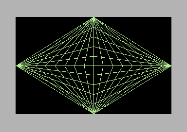
Download: Parabolic Star (Commodore 64 prg)

Download: Parabolic Star (source code)

 

 

 

As you can see from the source code, I had to implement both multiplications and divisions in assembly language. Those will be explained in detail on the next posts. The division routine is something I have come up with on my own and seems to work fine. The multiplication routine is a modified version of a routine by Jim Butterfield that I adapted to the size of the numbers used in the program. It should be fine as well. Now, let’s talk about the line drawing algorithm itself.

 

Standard line drawing algorithms make it possible to use integer unsigned numbers. Is it possible to use a standard mathematical approach (using continuous math and not numerical calculus) to draw lines with only integer unsigned numbers? The answer is definitely yes.

The equation of a line is:

y = m * x + q

Where m is the slope of the line, and q is a known term. You can see it as the equation of the function that we have to plot on the screen.

That equation doesn’t mean much for us in that generic form. Since we are going to draw a line joining two given points, we are better expressing the previous equation as follows:

y - y1 = m(x - x1)                           [1]

(x1, y1) is the starting point of the line, and (x,y) is a generic point of the line. (x,y) will change from (x1,y1) to (x2,y2) during line plotting. And (x2,y2), of course, is the end point of the line.

If we let x = x2 and y = y2, the slope m is:

m = (y2 - y1) / (x2 - x1)

Now, the basic concept here is that m can be evaluated by using integer division. Being a fractional number, evaluating it with integer division without a dangerous loss of accuracy requires an offset. So we can write:

m' = [(y2 - y1) * off ] / (x2 - x1)

The offset off is an integer number. The larger it will be, the more accuracy we will be blessed with. But of course, as long as the offset grows, we will have to deal with larger numbers.

Equation [1] above can be rewritten as:

y = m(x - x1) + y1 = m * x - m * x1 + y1

y = m * x - m * x1 + y1

Using m’ (the slope multiplied by the chosen offset), we have:

y = ( m' * x )/offset - (m' * x1) / offset + y1    [2]

This is the form that we must use. It allows not to loose much of the fractional information of the original m. Division by the offset is performed after multiplication: this is the trick.

One concern when plotting functions is continuity. If you have programmed function plotting, you will have noticed that sometimes points are not perfectly close to each other. There may be some “holes”.

On lines, it can happen depending on the slope.

Terms that make up the slope m are called “delta”. So:

m = (y2 - y1) / (x2 - x1) = deltay / deltax

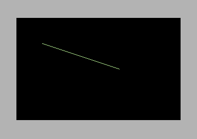
If deltax is greater than deltay, the equation:

y = m * x - m * x1 + y1                       (*)

will allow us to plot a line with points perfectly close to each other.

Instead, if deltax is lower then deltay, the equation will allow us to plot only a small set of points.

 

 

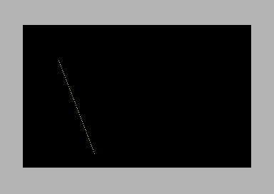
That demonstrates that equation (*) doesn’t work well if deltax is less than deltay.

But why that happens? Basically, there are not enough x points to obtain enough y points. And if y points are not enough, discontinuity happens.

We need more points to compute line points, but how we can add them? On a bitmapped screen, points can be only incremented by one, so the domain of the function is made up of a fixed amount of values. But, we can do this: we can calculate x points starting from y points. Take a look at the following equation:

x = m * y - m * y1 + x1                      (**)

 

By using this equation, since deltay is greater than deltax, we now have many y points. Now y points are the domain of the function, so we start from them. By using them, we can calculate many x  points, and the line will look continuous.

So, we must use two equations:

1)  y = m * x - m * x1 + y1        if deltax > deltay

2)  x = m * y - m * y1 + x1        if deltay > deltax

 

Please note that when using equation 2), m is calculated as:

m = deltax / deltay

 

Now, let’s talk about computational efficiency. Evaluating x or y values by using such equations is a little heavy, as we have multiplications.

When programming, each point will be calculated on a loop. If you look closely at the equations, only the terms m * x or m * y must be calculated on each iteration. The remaining terms, m * x1 and y1 or m * y1 and x1, are the same for each iteration. They are known from the beginning, as long as the terms m and y1 are known.

So, on each iteration we must only calculate m * x or m * y terms each time.

Still, we have to make a product on each iteration. But, we can actually use additions instead. While plotting lines, since we are moving from point to point by a step of one, we can make use of the fact that:

m * (x + 1 ) = m *x + m

As a result, we only need to calculate the product m * (x1) at the beginning. We can assign this product to a variable called mc. Then, when plotting the next point, we will add the term m to the variable mc. So:

m * (x + 1) = mc + m

on each iteration: mc = mc + m

This is quite similar to what the Bresenham algorithm does. Still, the global approach used here is totally different.

The above formula doesn’t take the offset into account. Now, we must deal with it.

As previously explained , the term m’ is:

m' = [(y2 - y1) * off ] / (x2 - x1)

Before the loop which draws the line, we must calculate:

MC = x1 * m'

We do not divide by offset at this stage.

On the first iteration inside the loop, we compute the first value of the term mx as follows:

MX = MC / offset

Then, we just increment MC:

MC = MC + m'

So, MC is the generic term m*x multiplied by offset. Each time, MC is incremented by m’. MC must NEVER by divided by offset in the statement: MC = MC + m’.

As you can see, this way we can use integer numbers and we can only perform additions inside the line drawing loop. Actually, there is a division (MX = MC / offset), but if the value of offset is chosen with care, this operation doesn’t even need shift/rotate instructions. It just requires simple and fast assignment instructions. Please see the source code of the Commodore 64 assembly version.

There’s still something that must be put clear: signs.

The bitmap screen we will be plotting lines on will be just a quadrant with both axes positive. So, our linear function will have a positive domain, and will produce positive values. This will be helpful to remember when dealing with signs.

The equation:

y = m * x - m * x1 + y1

is the generic form, where any term can hold a value both positive or negative. But, since we know both x and y terms are always positive, only the sign of m can change. And since m is the ratio between deltay and deltax (if deltax > deltay), the sign of m can be easily determined from the signs of both deltas.

Since we want to use unsigned numbers, we can actually split the above equations in two formulas, depending on the sign of m:

y = m * x - m * x1 + y1         (if m > 0)

y = - m * x + m * x1 + y1       (if m < 0)

But, to use unsigned numbers, we must rewrite those equations in a way that doesn’t produce negative values. So:

y = m * x + y1 - m * x1         (if m > 0)

y = m * x1 + y1 - m * x         (if m < 0)

We are sure signed numbers are not necessary here: y is positive, m is positive (e.g., we can take the module of it) because we are choosing the needed equation according to the sign of m. Operations are performed in the right sequence, so we have no negative partial results. Just as required. We have finally managed our target: integer unsigned numbers.

The following code, written in Commodore 64 BASIC, sums up all of the concepts. It is a part of a program I wrote to test my algorithm. Don’t run it.

116 m = int((dy*off)/dx)
117 if yn = 1 and xn = 1 then ms = 0
118 if yn = 0 and xn = 0 then ms = 0
119 if yn = 1 and xn = 0 then ms = 1
120 if yn = 0 and xn = 1 then ms = 1
122 s=1:if x2<x1 thens=-1
124 tt=int((x1*m)/of)
128 mc=int(x1*m)
130 forx=x1tox2steps
135 mx=int(mc/off)
140 ifms=0theny=y1+mx-tt
141 ifms=1theny=y1+tt-mx
143 mc=mc+(m*s)
145 gosub42:rem plot x,y
150 next

This piece of code deals with deltax > deltay.

yn and xn are variables that act as negative flags for deltay and deltax. A 0 value means positive, a 1 value means negative. Lines 117 from 120 determine the sign of m. As there is no XOR (exclusive OR) in Commodore 64 BASIC, I have implemented it by using some if statements. In 6502, the EOR instruction can be used instead. That’s much more straight.

ms holds the sign of m, and it allows to choose which formula to use.

s is used to determine the direction of the line. It depends on whether x1 is less than or greater than x2 (start point and end point of line respectively). I have used a signed value for this variable for the sake of clarity, but it is possible to modify the code and just select addition or subtraction when calculating MC.

Another part of the program computes deltax, deltay and sets flag signs accordingly. It also decides if calling the routine for deltax > deltay or the routine for deltax < deltay.

Mathematical details of the 6502/6510 implementation will be covered on the next posts. You may refer to this article for a simple introduction to 6502/6510 math.

Compared to most common line drawing algorithms, the approach used here has some disadvantages. First of all, the code is long and complex. Furthermore, sometimes lines don’t look too pretty (near the starting point or end point). Symmetry may also be of concern on some drawings. Still, slopes seem always to be quite exact here. On other algorithms, some corrections that make lines look better can actually alter slope at some degree.