The perspective drawing of a sphere coded in 6502 assembly language

Perspective drawing has always been fascinating to me. I will never stop being amazed at the wonder of seeing a 3D space perfectly rendered on a 2D plane, whether it is sheet of paper, or a video monitor.

Vectors is what you will always hear about while talking about 3D graphics principles. Still, it is possible to get a 3D view of an object even without using them.

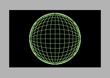
In this article, I will talk about an assembly language program I have been developing for the Commodore 64 in the latest few days. It draws a simple sphere with a chessboard texture on its surface. It looks like a wireframe sphere, but it uses very simple concepts.

 

DOWNLOAD: C64 Assembly Language Sphere – Source code

DOWNLOAD: C64 Assembly Language Sphere – Prg file

As it’s easy to see, the program draws various ellipses and a circle. It also draws a couple of lines. Each ellipse is drawn by using the equations:

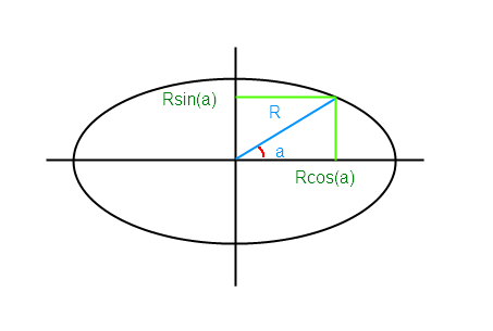
x = R1 * cos(a)
y = R2 * sin(a)

a = [0, 2 * PI]

 

When R1 = R2, you obtain a circle:

x = R * cos(a)
y = R * sin(a)

a = [0, 2 * PI]

 

These are parametric equations. a is the parameter, and it is assigned values from 0 to 2 * pi. In the equations of the circle, a has the proper meaning of “angle”. Generally, it is called a parameter.

Now, a sphere can be obtained by rotating a circle about an axis. For a solid sphere, this circle has infinite positions. But, we can imagine a sphere made up of a fixed number of circles, each one rotated at a certain angle. That way, you will have a “wireframe” sphere.

Ellipses are used to give a 3D effect. If you project a rotated circle on a plane, you obtain an ellipse. That’s the principle.

If the circle lies on a plane perpendicular to the projection plane, you won’t see an ellipse, but just a segment. That’s why two lines are drawn by the program.

The sphere is made up of two sets of circles:

• the circles rotated about the X axes;
• the circles rotated about the Y axes.

To draw the first set of circles (rotation about the X axes), R1 stays fixed (it is set to the sphere radius), while R2 changes for each ellipse. To draw the last set of circles, instead, R2 stays fixed while R1 changes.

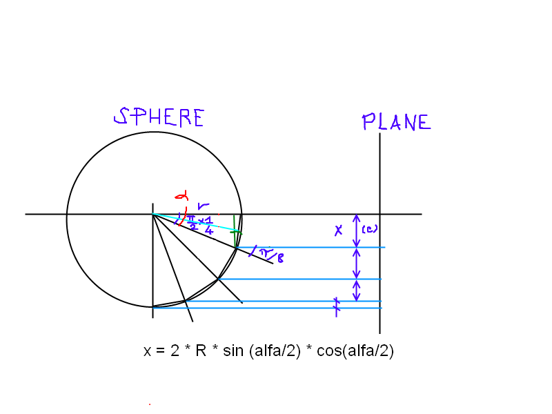
Values of the radii have been choosen so that you get a perspective effect. I have calculated them by simple trigonometric calculations, projecting each radius on a plane.

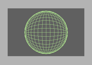
As Commodore 128 BASIC 7.0 do support ellipses, I made a simple program for the Commodore 128 showing off the above ideas.

2 rs=90:gosub40:graphic1,1
20 r1=rs:forr2=0to7:circle1,160,100,r1,ri(r2):next
30 r2=rs:forr1=0to6:circle1,160,100,ri(r1),r2:next
32 draw 1,160-rs,100 to 160+rs,100
33 draw 1,160,100-rs to 160,100+rs
34 poke 53280,15
35 geta$:ifa$=""then 35
37 graphic 0: poke 53280,13
39 end
40 print "radii:"
45 a=3.1415926/2/8:rem 8 edges
48 dim ri(7):cr=0
50 foran=atoa*8stepa
60 ri(cr)=2*(rs)*sin(an/2)*cos(an/2)
65 cr=cr+1
70 next
72 ri(6)=87
75 fort=0to7:printri(t):next
78 input "hit return";a$
80 return

 

 

Dowload: Sphere Commodore 128 BASIC

Commodore 128 BASIC implementation is quite straightforward. The CIRCLE instruction is very powerful. The sphere takes about 20 seconds to be drawn.

On the C128 program you can also see how radii have been calculated. The basic idea is explained on the following picture (on the picture, just a small number of radii has been used).

On the Commodore 64 assembly program, drawing the sphere takes only 6,7 seconds. This is because the C64 program uses mirroring to draw each ellipse. In facts, an ellipse is a symmetric figure. So, instead of calculating all the points, the program only calculates one quadrant of points, mirroring each point on the other quadrants.

A BASIC 2.0 implementation is possible, but it will be quite slow. Still, by using tables for sine and cosine functions it is possible to speed things up a little bit. Only 209 points per ellipse will be calculated: this way, ellipses will be plotted with very few points, but the program will be much faster.

 

Download: C64 BASIC versions of Sphere

One version is unbearably slow and doesn’t use tables. The second version takes advantage of tables and it is faster. Both programs are available in the above .d64 file.

 

Some thoughts on the Assembly Language version

I had many decisions to take in order to code this program. First of all, sin and cos functions evaluating.

The fastest way to compute trigonometric functions in assembler is by using tables. Now, the problem is, sinus and cosine functions produce values in the range -1 and 1. And those values are of course decimal. They are signed too. How do we manage to put a value such as -0.4657 in memory?

As we know, on any 8 bit system each RAM location can hold a value from 0 to 255. This value is an integer. What about the sign and decimal digits then?

To make the sign information available for each number, we can use the 2’s complement form. We can say that numbers between 0 and 127 are positve, and numbers from 255 and 128 are negative. So, -1 will be stored in memory as 255, -2 as 254 and so on.

Think about a tape counter. Typically, it can show numbers from 000 to 999. If you are on 000 and then rewind, you get 999, 998, 997 and so on. This is the same principle.

I have used a BASIC program to compute trigonometric functions values and to store them in memory by using two’s complement form. Then, the machine language program retrieves these values and converts them to “normal” values when needed.

Negative numbers are those bigger than 127. So, if the program loads a number with the value 255, it knows that it is negative and it must find its absolute value. The computation is fairly simple:

abs(x) = 256 - 255 = 1

The program must also set a “negative flag” to remember that the number loaded is negative. I am not talking about the negative flag of the CPU: it’s just a simple program variable that we make use of.

For example, to evaluate the Y value:

Y = 100 + R2 * sin(a)

If sin(a) is positive, we can just use the above formula. If it is negative (the flag will tell us), we will just have to use subtraction. And we will take the absolute value of sin(a). So, we will use this formula:

Y = 100 - R2 * abs(sin(a))

For example, if sin(a) is 253, the absolute value is 256-253 = 3. Evaluating the formula of Y, we will have to use subtraction because we know that 253 is a negative number.

The idea used in the machine language program is just this: to calculate Y = 100 + R2 * sin(a),  take the module of the value sin(a) if needed (if sin(a) is positive, then just take the value), set the flag to 0 or 1 depending if the original value is either potive or negative, perform the multiplication (R2 * abs(sin(a) or R2 * sin(a)), then add the result to 100 or subtract it from 100 depending to the value of the flag.

We could also use another approach. We could use the same formula for either positive and negative numbers. But that would require converting to the 2’s complement form the product R2 * abs(sin(a)). For simple formulas like the ones used on this program, using two separate formulas to keep signs into account is much simpler and efficient I think.

Now to the decimal digits issue. We will not use fixed point numbers, nor floating point numbers. Integer numbers are enough to hold decimal digits. But we must use an offset. To create the table, we must evaluate sin(a), for each value of a, then we must multiply it by an offset (the value 128 in this program). The table will be made up of sinus and cosines values multiplied by 128.

The machine language program may then just load those values and divide them by 128. Dividing by 128, being a power of 2, is just a matter of simple shift instructions (that’s why I have choosen such an offset). The bigger the offset, the more “decimal numbers information” will be preserved.

But, dividing by 128 the value of the table is useless. As we handle integer numbers, we would only get 0 or 1. But, we can do this:

Y = (sin_table_value * R2)/128

For general math, it is the same as Y = (sin_table_value / 128) * R2, but for us, it is definetely not, as we are working with integers.

This way, we will have the decimal digits information preserved even if using integer numbers.

For example:

sin(0.4) = 0,389
sin(0.4) * R = sin(0.4) * 50 = 20

sin(0.4) = 0,389
table_value(0.4) = 0,389 * 128 = 49 (integer value)
sin(0.4) * R = (table_value(0.4) * 50)/ 128 = 
= (49 * 50)/128 = 19 (integer value)

sin(0.4) * R = (table_value(0.4) / 128) * 50 = 0 (wrong!)

By performing multiplications and additions in the right sequence, the method works. The approximate value of the sinus function (19) is of course different from the real value (20), but this difference is acceptable for our purposes. After all, we will be plotting on a screen with 320 x 200 dots.

For more precision, the offset may be increased. But 128 works good enough for us. It allows for 8 bit numbers on the table, and that will make computations faster in the program.

On the next posts, I will talk about 6502 assembly math and hi-res screen plotting in machine language, so that further explanations about the machine language Sphere program will be provided.