Another look at 3D graphics: fast hidden faces removal (back-face culling)

While doing even very simple 3D graphics, the need of a better rendering of images will soon arise. Wireframe 3D objects with all lines drawn will look confusing. So, some way of removing hidden faces must be found. And, since this blog actually deals with retrocomputers, we also need a fast way to do that.

On this article, I somewhat managed to come up with a very simple algorithm that was able to handle the hidden lines problem, but only dealing with a particular situation (x axis rotation of a cube). Now, we are going to find a general answer to the problem. This way, we will be able to hide the surfaces of a generic 3D object with any orientation in the space.

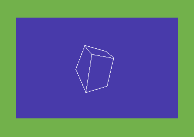
The following program for the Commodore 64 will rotate a cube featuring a hidden faces removal technique. General principles will be explained so that experiments with any other computer and/or programming language will be possible.

 

Download: Commodore 64 rotating cube, hidden surfaces (prg file)

Download: Commodore 64 rotating cube, hidden surfaces (source code)

 

 

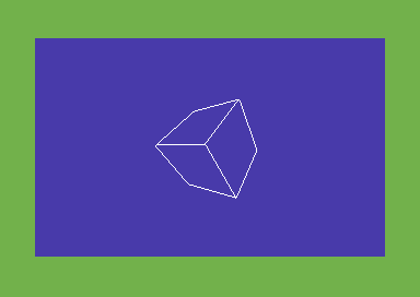
Confusing hidden lines are now gone. This way, no optical illusions happen. Of course, this is a simple wireframe rendering with no colors and shades, but still, you now get a good idea of how the real object would look.

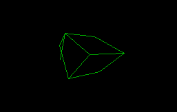
A cube is relatively easy to handle, as it has no tilted surfaces. As it will be explained later, if an object has tilted surfaces, hidden surfaces removal is a bit more difficult (at least, using the fast technique that will be discussed in a moment). So, the following program is more general.

 

Download: 3D object with inclined surface (prg file)

Download: 3D object with inclined surface (source code)

 

 

There is quite a bit of math inside these simple routines. So, I am going to provide you with a hopefully detailed explanation of  the theory involved.

 

Projections and visibility of faces

 

The above programs use slightly different projections equations than my previous 3D programs with no general hidden surfaces removal algorithm. These are:

x1 = d*x/(z-z0)	
y1 = d*y/(z-z0)

Here, a distance d and a translation amount z0 are introduced.

In a nutshell, d can be seen as a zooming factor, while z0 acts as the z coordinate of the COP (center of projection). z0 must be chosen so that z-z0 < 0.

The z0 parameter is quite important, as it is related to the concept of visibility of a projected surface.

As you may remember from my old x-rotating cube program with hidden lines removal, a “prospective angle” was introduced. Well, that angle is due to projections. On orthogonal projections, that would be not needed. And that angle is just related to z0. This concept will be useful in a moment.

 

Normal vector of a surface

 

If we want to decide whether a surface is visible or not, we need some way of establishing its orientation in the space. To do that, a normal vector to the surface is used.

A normal vector is any vector that forms a 90 degrees angle with the surface. Of course, we are dealing with flat surfaces.

 

 

Those in red are examples of normal vectors of flat surfaces. For instance, N1 is the normal vector of surface 1.

How do we compute normal vectors? On a cube, we don’t really need to compute them. To establish the orientation of a surface we just need any normal vector. And, for instance, AB is just a normal vector for surface 1.

So, an edge of a cube can act as a normal vector for a given surface. That’s why normal vectors calculations are not needed in such a case.

But in general, the normal vector of a tilted surface must be evaluated. To do that, we need the cross product, an operation between two vectors that gives another vector.

 

Cross product

Given two vectors V1 and V2 lying on the same plane, the cross product between them gives another vector V3 that is perpendicular to that plane.

So, if we take two vectors that lie on a surface, the cross product will give us a normal vector to that surface. That’s just what we are looking for.

Given the two vectors AB and AC, their cross product is:

AB X AC = V

Now, we have to evaluate the coordinates of V.

If the coordinates to the origin of the points A, B and C are as follows:

A = (xa, ya, za); B = (xb, yb, zb); C = (xc, yc, zc)

then, the vectors AB and AC will have coordinates:

AB = (xb-xa, yb-ya, zb-za) = (xba, yba, zba)

AC = (xc-xa, yc-ya, zc-za) = (xca, yca, zca)

Given two vectors, V1 = (x1, y1, z1) and V2 = (x2, y2, z2), the cross product gives a vector with the following components:

V1 x V2 = V = (y1*z2-y2*z1, x2*z1-x1*z2, x1*y2 - x2*y1)

So, we have:

AB x AC = V =(yba*zca - yca*zba, xca*zba - xba*zca, yba*yca-xca*yba)

The components of V are then the components of a vector which is normal to our surface.

As you may have noticed, the vector V is much longer than both AB and AC. We are dealing with a product, and its length is actually proportional to |AB|*|AC|. Since we must use the endpoint of V for calculations, we definitely need a smaller vector which is parallel to V. To obtain such a vector, we may scale down V. But, such an operation requires some care.

 

Scaling a vector: multiplying a vector by a number

 

If we take the components of V and we multiply them all by a number, then we are scaling the vector V by a factor number.

So, we can multiply each component for a number lower than 1 to scale the vector down.

But, if we just scale the normal vector V down, we obtain a new vector that is no longer applied to the point A (that means, A is no longer the starting point of vector V, seen as a segment).

In the following pictures, the vector V is applied to the point O (instead of A), the center of the surface. Concepts don’t change.

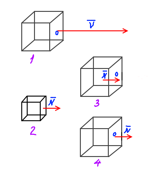
Picture 1 shows the cross product vector V applied to the center point of the surface. It just makes a too bigger normal vector.

If we scale down both the cube and the vector V, we obtain a normal vector N which is smaller than V and which is still applied to the center point of the surface. But, we don’t want to scale down the cube.

If we only scale down the vector V, we have a side effect: the vector N is no longer applied to the surface, so it is useless.

We just need what happens in picture 4: the scaled down vector must be kept applied to the surface. That way, it will be able to represent its orientation on space.

If we scale down the vector V till it reaches 0, we would want it to be applied to the surface anyway. So, if the point O where the normal vector is applied has coordinates xO, yO, zO, then the scaled down normal vector can be obtained as:

N = (vx * sf + xO, vy*sf + yO, vz*sf + zO)

Where:

sf = scale factor, a fractional number lower than 1 and bigger than 0;

vx, vy, vz = coordinates of the vector V

N = normal vector to the surface

xO, yO, zO = coordinates of the point where the normal vector is applied.

It’s easy to see that by using the above formula, if vx, vy and vz are all 0, we have N = (xO, yO, zO). So, no matter how much we scale down the vector V, if we use the above formula, it will be always applied to the point O.

 

Visibility of a surface – dot product

 

Imagine that you have a line starting from the screen you are just viewing. This line is perpendicular to the screen. A vector B is parallel to this line.

Suppose you are watching a rotating cube. In particular, you are watching a surface of it. This surface has a normal vector N.

 

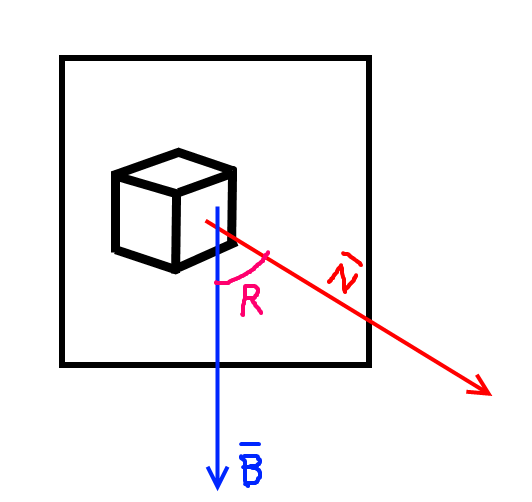
If the angle R between B and N is in the -90/+90 degrees range, the surface will be visible. Otherwise, the surface will be hidden.

Now, we must find a formula that tells us in what range the angle R is.

The dot product between two vectors is a number. Given two vectors V1 and V2, the dot product is:

V1 . V2 = |V1|*|V2|*cos(R)

Where R is the angle between the two vectors, like in the above picture.

Given the behaviour of the cosine function, it’s easy to see that the angle R will be in the range -90/+90 degrees only when the dot product will be positive.

So, if the dot product between the vectors B and N is positive, then the surface is visible. Otherwise, if the dot product between the vectors B and N is negative, then the surface will be hidden.

The dot product can be also expressed using the coordinates of the two vectors involved in the product. So, given two vectors V1 and V2 with coordinates V1 = (x1, y1, z1) and V2 = (x2, y2, z2), the dot product between them is:

V1 . V2 = (x1*x2+y1*y2+z1*z2)

So, to check for visibility, we need to evaluate the dot product using this last formula, then we have to check the sign of it.

The above visibility relation is true only for orthogonal projections. For prospective projections, this formula must be adjusted.

 

Visibility check with perspective

 

When our 3D  object is represented on screen by using orthogonal projection, the straight dot product B . N can be used to check for visibility of a surface with normal vector N.

If we look at the front of a cube, with a zero rotation angle, by using orthogonal projections we just see a square. Even if we want to draw hidden lines, we just can’t, as they perfectly overlap with visible lines.

 

If we look at the front of the cube with perspective projections instead, hidden lines can be drawn. The front face of the cube is the bigger square, the opposite face is the smaller square.

Perspective changes the way visibility of surfaces must be checked. For instance, if we rotate the cube by a very little amount, results will change depending on the projection method.

When using orthogonal projections, even if we rotate the cube by a very small amount, two faces are visible on the screen.

Instead, if we use perspective projections, if we rotate the cube by a very small amount, only one face will be visible. So, we cannot use the visibility relation used for orthogonal projections. Otherwise, hidden lines would be shown.

We still have to evaluate the sign of a dot product, but vector B must be changed. We need a vector that keeps the projection method into account.

So, instead of B, we use a vector that starts from a point on the surface and ends to the COP (center of projection). So, the new visibility relation is:

Visibility = N . PCOP > 0

Where P is any point on the surface of which to check visibility. PCOP is a vector from P to the COP.

 

 

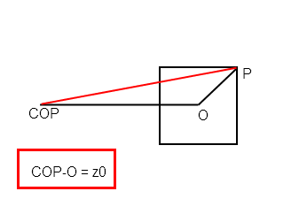
From the above picture, we can clearly see that the vector PCOP is made up of two vectors: COPO and PO (O is the origin). Please note that the length of COPO equals z0, which was used in the projection equations.

So, the visibility relation can be rewritten as:

Visibility = N . PCOP = N . (COPO + PO) > 0

Where:

COPO = (0, 0,-z0)

PO = (Px,Py,Pz)

So:

Visibility = N . COPO + N . PO = -Nz*z0 + N . PO > 0

Since we have a rigid solid performing rigid rotations,  the modules of N  and PO never change. The angle between them does not change either. Furthermore, the term z0 is also a constant. So, we can use the following constant:

K =  (N . PO) / z0

So, the visibility relation simply becomes:

Visibility = K - Nz > 0

That means, we only need the length of the normal vector along the z axis and the constant K to check visibility. We don’t need to take the dot product each time to check for face visibility. That means a great computational advantage.

Nz can be obtained by:

Nz = Z(P1) - Z(P2)

Where P1 is the point the normal vector starts from, P2 is the point where the normal vector ends. So, to evaluate Nz we just need a couple of z components. So, we finally have:

Visibility = K - Z(P1) + Z(P2) > 0

 

This is the relation used in the code. There is only a little difference. As normal vectors are chosen to point towards the inside of the object, the “>” operator is actually inverted in the code.

 

How to compute z constants – Visibility checks

For a cube, due to its symmetry and its flat surfaces, we only need one K constant.

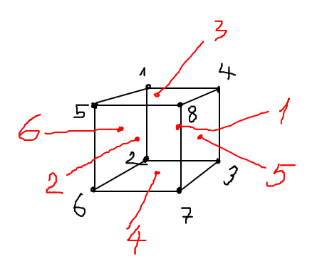
To compute K, we just need to choose a point on a surface, and a normal vector for that surface. Let’s take for example face 1. We can take the point 1 as a point of the surface, and the vector 15  as the normal vector.

From the code, we have the following coordinates:

P1 = (p1x, p1y, p1z) = (-L, -L, -L)

P5 = (p5x, p5y, p5z) = (-L, -L, L)

with L = 70, z0 = 150.

So, we have:

K = (p1x * (p1x - p5x) + p1y * (p1y- p5y) + p1z * (p1z - p5z))/z0

K = 16.33

To check visibility of face 1, we only need the simple relation:

vis = k - z(1) + z(5)

And we must check if vis < 0 for surface visibility.

 

If we have a surface with slope, we need to compute the normal vector.

First of all, we have to find two vectors that lie on the surface. For instance, vectors 56 and 58. Those have components:

x1 = (x(5)-x(6))
y1 = (y(5)-y(6))
z1 = (z(5)-z(6))

x2 = (x(5)-x(8))
y2 = (y(5)-y(8))
z2 = (z(5)-z(8))

The normal vector is the cross product between them. Its components are:

xn = y1*z2-y2*z1
yn = -(x1*x2-x2*z1)
zn = x1*y2-x2*y1

Now, we need to scale down the normal vector. Since 56 and 58 have point 5 in common, the normal vector is applied to point 5. So, to scale down that vector we have:

x(9) = xn*0.010+x(5) 
y(9) = yn*0.010+y(5)
z(9) = zn*0.010+z(5)

Now, point 9 is the end point of the normal vector. 0.010 is the scale factor.

Please note that x(9) must be rotated along with the other points. It will not be plotted but it must be regarded as a point of the solid. That means, x(9) must be computed only once. Then, we just rotate it along with all other points, and we will always have the normal vector of the surface, with points 5 and 9.

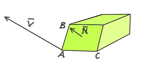
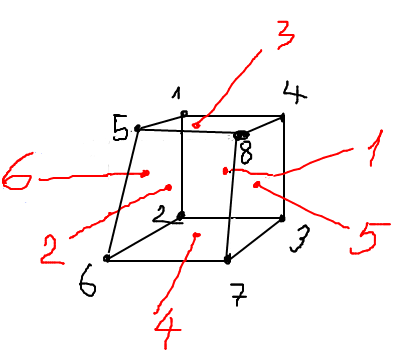
The following picture shows the normal vector to the surface with slope.

 

 

The K constant to use with the inclined surface (let’s call it k2), can be computed as:

k2 = (x(5)*(x(5)-x(9))+y(5)*(y(5)-y(9))+z(5)*(z(5)-z(9)))/z0

Please note that we also have to recalculate the K constant for the other surfaces, as point 5 has now changed. So, using face 5:

k = (x(4) * (x(4)-x(1)) + y(4)*(y(4)-y(1)) + z(4)*(z(4)-z(1)))/z0

The previous value of K now only works for the surface opposite to the inclined surface, let’s call it K3. That’s because the distance from point 5 and the origin has changed:

k3 = (x(1) * (x(1)-x(5)) + y(1)*(y(1)-y(5)) + z(1)*(z(1)-z(5)))/z0

One thing is important to note: we must select the point to which we apply the normal vector for visibility check according to what we have done when computing K.

For instance, to compute K for the cube, we have chosen a vertex, then the normal vector starting from that vertex. So, for the visibility check, we must use a vertex as well – that is, a point which has the same distance from the origin. This is required to stay in tune with the previously written equation:

Visibility = N . COPO + N . PO = -Nz*z0 + N . PO > 0

Now we are done. To check for visibility of the inclined surface, we will use the relation:

vis = k2 - z(5) + z(9)

To check for visibility of the face opposite to it:

vis = k3 - z(1) + z(5)

For all other faces, we will just use K and we will choose the normal vectors like on the cube.

 

Some words about the code

The code of the programs presented at the beginning should be quite clear now. Please note that visibility is computed using 16 bit numbers. That is required to avoid signed overflow. We could check for overflow, but this way code is much simple.

For instance, visibility check for face 1 of the cube goes like this:

;computes visibility of face 1 

                lda #$00
                sta za
                sta zb                  ;resets high bytes 

                ldy #0
                lda zd_component,y 
                sta za+1
                bpl skip_neg 
                
                lda #$ff
                sta za                  ;set high byte to $ff for negative value of 16 bit number za 
                                        ;else it stays to zero 
skip_neg        ldy #4
                lda zd_component,y 
                sta zb+1
                bpl skip_neg2 
                
                lda #$ff
                sta zb       
skip_neg2       
                sec
                lda k+1
                sbc za+1
                sta vis+1
                lda k
                sbc za 
                sta vis                 ;vis = k-za

                clc 
                lda vis+1
                adc zb+1
                sta vis+1
                lda vis 
                adc zb 
                sta vis                 ;vis = vis + kb = k-za+zb 
                
                bpl skip_face1 

 

As tables in the assembly code start from index 0, we need to subtract a 1 to point numbers. So, points 1 and 5 from the pictures are replaced with points 0 and 4 in the code.

K constants are 16 bit with high byte set to 0.

For the cube program:

k byte 0,16 ;constant used for hidden surfaces

While for the solid with inclined surface, we need three constants:

k byte 0,16 ;constants used for hidden surfaces 
k2 byte 0,6
k3 byte 0,8

 

Despite the code is not optimal, those checks are quite fast. Actually, the programs with hidden lines removal run no slower than the older versions showing all lines.

Things are arranged so that common lines are not drawn twice. The flags face1, face2, face3 and face4 are used for the purpose.

 

References

• A Different Perspective, part II
• Back face removal.
• Wikipedia entries for dot product and cross product.