Note: although the concepts of circle and circumference are different, we will often use here the term “circle”, although we are actually referring to the circumference.
Definition of a circle
A circle with center C and radius R is a set of points that can be represented as follows:
C = [ P / CP = R ]
which means: the circumference is made up of any point P which has a distance from the center of the circumference that equals a fixed amount R (the radius of the circle).
The center C has coordinates x0 and y0.
The condition CP = R can be written as:
SQR((x-x0)^2+(y-y0)^2) = R
Squaring both terms of the previous equation:
(x-x0)^2+(y-y0)^2 = R^2
This is the equation of the circumference with center C(x0, y0) and radius R.
By expanding the above equation we obtain:
    x^2 - 2 * x0 * x + x0^2 + y^2 - 2* y0 * y + y0^2 = R^2

(1) x^2 + y^2 - 2 *x0 * x - 2 * y0 * y + x0^2 + y0^ 2 - R^2 = 0
If we want a more compact form, let:
- 2 * x0 = A
- 2 * y0 = B
x0^2 + y0^2 - R^2 = C
So, the equation becomes:
(2) x^2 + y^2 +A * x + B * y + C = 0
Although (2) is more compact, (1) is what is more useful for programming, as center points and radius can be obtained directly.
Equations for drawing a circle
Equations (1) or (2) are given in the implicit form. That means, those cannot be used for drawing a circle. For that, we need an explicit form.
Starting from equation (1), if we solve it to y we obtain:
(a)     y1 = -(SQR(R^2-x^2+2*x0*x-x0^2) - y0

(b)     y2 = SQR(R^2-x^2+2*x0*x-x0^2) + y0
Those equations are in the y = f(x) explicit form.
But we also need the equations in the x=f(y) explicit form:
(c)     x1 = -(SQR(R^2-y^2+2*y0*y-y0^2) -x0

(d)     x2 = SQR(R^2-y^2+2*y0*y-y0^2) +x0
If we want to use those expressions to plot a circle, we need BOTH explicit forms (y=f(x) and x=f(y)).
(a) and (b) combined allow to plot a circle. The same goes for (c) and (d) combined. And, both couples allow to plot the same circle.
But, if we use equations (a) and (b), here’s what we get with Simons’ BASIC (Commodore 64):
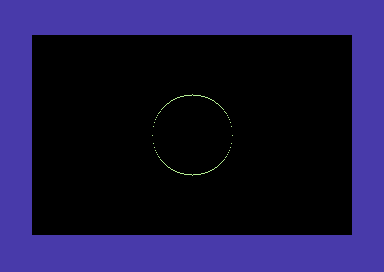
Domain of the function: X values between x0-R and x0 + R.
As it’s easy to see, we have many missing points. Those points are around a horizontal line passing to the center of the circle.
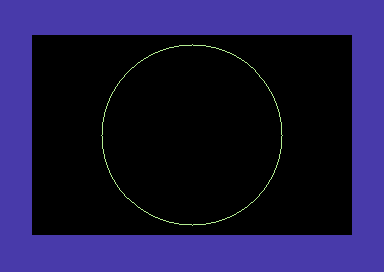
If we use equations (c) and (d), we obtain instead:
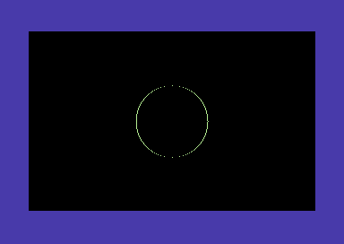
Domain of the function: Y values from y0-R and y0+R.
Now, missing points are around a vertical line passing to the center of the circle.
The code is as follows:
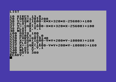
These are actually two programs. If you start the program with RUN, you get the circle with equations (a) and (b). With RUN 210 you obtain the circle given by equations (c) and (d).
Why do we get discontinuity? Because we are using equations based on continuity (infinite points) on a bitmap screen which has only discrete points.
The only solution to get continuity is to draw the circle by using both couples (a), (b) and (c),(d). Each equations couple will be used where it works the best.
For lines, the explicit form y=f(x) works well only when dx > dy. If dy > dx, we have to use the form x =f(y). The same applies to tangent lines of a circumference. And since the equations of tangent lines can be obtained by differentiating the equation of the circumference, it’s clear that continuity on the circumference equations works the same as continuity on line equations.
So, we can determine the transition points between the parts of the circle where we have to use equations (a) and (b) (y=f(x)), and the parts where we have to use the equations (c) and (d) (x=f(y)).
Transition points are just those points of the circle where we have a tangent line with a 45 degrees slope (dx = dy, using the deltas for lines).

Red lines are all tangents to the circumference on the transitions points (blue points, TP).
From trigonometry, it’s easy to see that:
XTP = R * cos(a)

YTP = R * sin(a)
So, it’s easy to obtain the coordinates of the transitions points. Those will be used to build the domains for the explicit functions of the circumference curves (like on the code that follows).
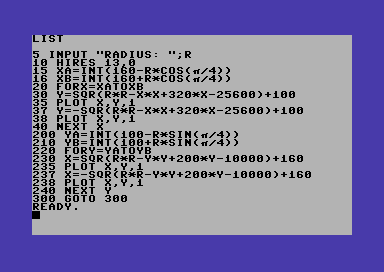
Download (requires Simons’ BASIC).
NOTE: the code needs optimizing to best handle continuity near transition points – please see this article.
The circumference is centered at (160, 100). This is the center of the bitmap screen.
Half part of the circumference is drawn by using equations (a), (b), using the domain X : [XA…. XB]. The other half is drawn by using equations (c), (d), with the domain Y : [YA… YB].