An introduction to vector-based graphics on the Commodore 64 – Rotating simple 3D objects (assembly language)

Vector-based graphics or 3D graphics is quite common today. On old 8 bit computers it was not very common instead, due to the large amount of computing power required to render even simple objects. Despite some 3D software was available for 8 bit systems, most software made use of 2D graphics only. Still, 3D routines are quite common on today’s C64 scene productions. In facts, 3D is a good play field for talented coders wanting to go beyond the limits of the Commodore 64. But, this is not what we are going to achieve here. We will just have a look at the principles, and we will discuss some very simple assembly implementations.

On this article, we had a look at the principles behind 3D graphics, and we crudely defined a 3D vector as a set of three coordinates representing a point in the space. Once points have been projected in the plane (the screen), 3D objects can be simply drawn by joining these points with lines.

Coding a 3D routine in assembly is not that difficult (if you don’t want excellent performances), still many decisions must be taken. We definitely need signed fractional numbers. And if we want speed, we cannot use floating point numbers. So, like on other programs, we will use integer numbers in two’s complement form and we will rely on integer math.

On my previous 3D article I had shown a simple Freebasic implementation of a rotating cube algorithm. Before coding the C64 assembly version, I have had a look at that program and I have changed it so that it could support integer math. The result is the following Freebasic code, that just resembles closely what the C64 assembly version will look like. So, all the principles needed to code the assembly version are there.

rem rotating cube - freebasic

screen 13

dim as integer l, fs, c, s

dim x (1 to 8) as integer
dim y (1 to 8) as integer
dim z (1 to 8) as integer
dim pf (0 to 255) as integer
dim nf (0 to 255) as integer
dim as integer co(0 to 100), si(0 to 100)

dim xd (1 to 8) as integer
dim yd (1 to 8) as integer
dim zd (1 to 8) as integer

dim as integer xt, yt, zt

dim np as integer

dim offset as integer

dim as integer k, rx

dim kx as single

dim as integer vx(1 to 8), vy(1 to 8)

offset = 64

rx = 0 : rem rotation angle x

l = 80 : fs = 200 : l = l /2


for kx = 0 to 6.28 step .1

 co(rx) = int(offset*cos(kx))
 si(rx) = int(offset*sin(kx))
 
 rx = rx + 1
 
next kx


for k = 0 to 190


 pf (k) = (fs*offset)/(k+fs)
 
 nf (k) = (fs*offset)/(fs-k)
 
next


rx = 0

x(1) = -l : y(1) = -l : z(1) = -l
x(2) = -l: y(2) = l: z(2) = -l
x(3) = l: y(3) = l: z(3) = -l
x(4) = l : y(4) = -l : z(4) = -l
x(5) = -l : y(5) = -l: z(5) = l
x(6) = -l : y(6) = l: z(6) = l
x(7) = l: y(7) = l: z(7) = l
x(8) = l: y(8) = -l: z(8) = l


label_35:

 cls
 

 c = co(rx): s = si(rx)
 
 for np = 1 to 8

 rem rotation on x axes

 yt = y(np) 
 
 yd(np) = (c*yt-s*z(np))/offset: zd(np) =(s*yt + c*z(np))/offset


 rem rotation on y axes


 xt = x(np): zt = zd(np)

 xd(np) = (c*xt+s*zt)/offset: zd(np)=(c*zt-s*xt)/offset

 rem rotation on z axes


 xt = xd(np): yt = yd(np) 
 
 xd(np)=(c*xt-s*yt)/offset : yd(np) = (s*xt+c*yt)/offset



 rem points projections and translations to screen coordinates
 
 
 
 if zd(np) < 0 then

 vx(np) = 160 + (xd(np) * nf(abs(zd(np))))/offset
 
 vy(np) = 100 + (yd(np) * nf(abs(zd(np))))/offset
 
 
 else 
 
 vx(np) = 160 + (xd(np) * pf(zd(np)))/offset

 vy(np) = 100 + (yd(np) * pf(zd(np)))/offset
 
 end if 
 
 rem vx(np) = 160 + (x(np)*fs)/(z(np)+fs)
 rem vy(np) = 100 + (y(np)*fs)/(z(np)+fs)


next


line (vx(1), vy(1))-(vx(2),vy(2)),2 : line (vx(2), vy(2)) - (vx(3), vy(3)), 2 
line (vx(3), vy(3))-(vx(4),vy(4)),2 : line (vx(4), vy(4)) - (vx(1), vy(1)), 2
line (vx(5), vy(5))-(vx(6),vy(6)),2 : line (vx(6), vy(6)) - (vx(7), vy(7)), 2
line (vx(7), vy(7))-(vx(8),vy(8)),2 : line (vx(8), vy(8)) - (vx(5), vy(5)), 2
line (vx(1), vy(1)) - (vx(5), vy(5)), 2
line (vx(4), vy(4))-(vx(8),vy(8)),2 : line (vx(2), vy(2)) - (vx(6), vy(6)), 2
line (vx(3), vy(3))-(vx(7),vy(7)),2

sleep 50


rx = rx + 1 : if rx > 62 then rx = 0

goto label_35

 

On each rotating loop, the program takes the initial points and rotates them by an increasing angle. This is better than using previously rotated points to perform a new rotation, using a small fixed angle. That approach would actually result in an accuracy loss, since the approximation errors of the rotations tend to accumulate. If we just take the initial points for each rotation, no errors will accumulate. So, the rotation angle grows on each iteration by a little, fixed amount.

The program starts by creating some tables. Trig tables are simply created using the offset (64):

co(rx) = int(offset*cos(kx))

So, fractional numbers are translated into integer numbers. Two’s complement form is not used here, but it will be used in the assembly program.

The program then creates projection tables. Those are used to quickly project 3D points in the plane, without having to resort on division.

For example, to project a point we should use a relation such as:

vx(np) = 160 + (x(np)*fs)/(z(np)+fs)

That asks for a division. But, the above expression can be rewritten as:

vx(np) = 160 + x(np) * (fs/(z(np)+fs))

So, we can just create a table with the value of the term (fs/(zn(np)+fs)) for each Z. Since we are only going to use eight bit numbers, such a table is quite short. So, we gain speed without too much memory waste. Please note that two tables have been created. One for negative z, and one for positive z. To keep the code simple, we will just use the module of z as an index to look for the projection factor in the table. The sign of z will determine which table to use.

Notice the use of integer math to compute the projection factors.

The rotation angle is initially set to 0. After sine and cosine of rotation angle are taken, the rotation loop starts.

Rotations are performed using working coordinates (xd, yd, zd). Initial coordinates are never changed. This is an improvement over the previous version (please see this article): this way, values must not be retrieved before each rotation. To make things work fine, temporary storage locations must be used (xt, yt, zt). As each rotation requires two formulas, it may happen that the first formula transforms a coordinate that the second formula needs in its original form. Hence the need of temporary variables. Even when they are not mandatory, they are still useful to retrieve values faster.

We don’t  use a rotation matrix for all rotations. We just use a formula for each rotation. This is not efficient, but still, it allows to keep things simple.

After all eight points of the cube are rotated, it’s time to project them on the plane. The sign of Z is checked, then the projection term is retrieved from the right table using the module of Z.

After lines are plotted, the rotation angle is increased (actually, it is the index to trigonometric tables), then the process starts again. As values of trigonometric functions repeat themselves, when it goes past its maximum value the rotation angle is reset to 0.

 

Commodore 64 assembly implementation

 

One thing that is needed for 3D routines is a fast line-drawing routine. The line drawing routine I presented some time ago was just an experiment. It is reasonably fast (when compared to some line drawing routines like the ones in Simon’s BASIC), but it is not fast enough for vector graphics. I just wanted to show myself that, by just using integer unsigned numbers, it is possible to draw lines by using the equation of the line (y = mx + q), but that’s just plotting a linear function, something that can’t be as efficient as a Bresenham style algorithm.

On the article “A different Perspective: part 1” in Commodore Hacking, I have found some nice code for a quick line drawing routine. I didn’t look at the code in the main program presented there, I just looked at the piece of code presented in the “theory”, then I came up with my own version. It’s not a very fast line drawing routine, but still it performs better than my old version. I could re-use a part of my old code however.

The following code handles the case when DX > DY (please refer to this article for more details on line drawing routines).

 

;subroutine: fast line 

		;based on v1.3 SLJ 7/2/94
                ;x is only 8 bit - for the cube program is enough 
                
                lda #$00
                sta x2
                sta x1                                  ;set high bytes to zero
                sta xp 
                sta accumulator                         ;zeroes accumulator for line drawing 
                
                lda     x2+1 
                sta     limit
                
                lda     x_n 
                bne     dec_limit
                
                inc     limit 
                jmp     skip_dec_limit 
                
dec_limit       dec     limit 
                
skip_dec_limit  sec
                LDA	accumulator              
                SBC     delta_x+1 
                sta     accumulator
                
LOOPL           jsr     plot 
                               
                lda     x_n 
                bne     dec_x                           ;checks for delta_x sign  

                INC     x1+1	                        ;Step in x
                jmp     skip_dec_x 
                
dec_x           DEC     x1+1 

skip_dec_x      clc
                lda     accumulator 
                ADC	delta_y	                        ;Add DY
                sta     accumulator 
                BCC     NOPE	                        ;Time to step in y?
                
                lda     y_n
                bne     dec_y
                
                INC	y1	                        ;Step in y
                
                jmp     skip_dec_y
                
dec_y           dec     y1 
                
skip_dec_y      
                
                SEC 
                LDA     accumulator 
                SBC	delta_x+1	                ;Reset counter
                sta     accumulator 
                
NOPE            

                
                lda     x1+1
                cmp     limit 	                        ;At the endpoint yet?
                bne	LOOPL                            
                
                RTS

 

This routine doesn’t require to compute the slope of the line. It just uses the terms DX and DY in a clever way. On each iteration, x value is incremented by one. At a certain point, a step in the y direction must be taken. The variable accumulator determines when it’s time to take a step in the y direction. At the beginning, accumulator is initialized by storing -DX on it. Then, it is incremented by the term DY each time x is incremented by 1. When accumulator wraps around to zero, we know it’s time to increment y. In a way, we make use of the slope of the line even if we don’t know it. As the slope it’s just the ratio between the terms  DY and DX, accumulator wraps around to zero with a frequency that just depends on the slope of the line. That’s why the above routine works.

The above code works only when DX > DY, DX>0 and DY>0. Another routine for DY>DX must be created. Furthermore, the sign of DX and DY must be checked, so that the starting value of X or Y is either increased or decreased (the flag x_n is used in the above code). The code that you will find in my 3D programs handles all of this: it determines what routine to use (DX > DY or DY > DX), and checks signs of these terms.

This code is by no means optimal. I just wanted something a bit faster than my previous code and easy to use on various programs.

Now that we have developed a faster line drawing routine and we have coded an integer math 3D BASIC program, we just have all that is required to create an assembly version of the rotating cube program.

 

NOTE: updated versions (19/02/2018).

 

DOWNLOAD: 3D cube, x axis rotation (prg file)

DOWNLOAD: 3D cube, x axis rotation (source code)

 

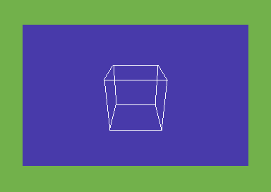
The above program performs a rotation about the x axis of a cube. Please note that all lines are visible (including hidden lines, that is lines that are out of our point of view). That implies an imperfect rendering of the cube, and it may appear deformed at times. That is just an aliasing effect due to an optical illusion. Sometimes the cube seems to rotate in the opposite direction and appears deformed. It’s just that our brain sees its shape in the wrong way at times. When you feel you’re seeing something strange, just pause the program (when using VICE, use the pause function) and look at the image: you’ll see that it is actually correct. This happens because hidden lines have been drawn, resulting in some hidden surfaces actually being shown that can trick our brain.

The following versions (still showing both visible and hidden lines), perform rotations about other axis, and show a bigger cube.

 

DOWNLOAD: 3D cube, x axis rotation, bigger (prg file)

DOWNLOAD: 3D cube, x axis rotation, bigger (source code)

 

 

 

DOWNLOAD: 3D cube, y axis rotation, bigger (prg file)

DOWNLOAD: 3D cube, y axis rotation, bigger (source code)

 

 

 

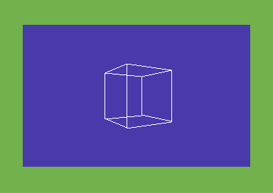
DOWNLOAD: 3D cube, x-y axis rotation, bigger (prg file)

DOWNLOAD: 3D cube, x-y axis rotation, bigger (source code)

 

 

A general hidden-lines removal routine is quite complex, and asks for the use of concepts like normal vector, cross product, dot product and so on (you may have a look at this article for details). Without bothering with those mathematical concepts, I just came up with a rude algorithm that works with the x-axis rotation. It is based on the idea that lines to be showed can be selected depending on the value of the rotation angle. That is, for a given range of rotation angles, some lines must be showed, others must not. The following sketch that I did in a hurry while coding hopefully shows my idea.

 

 

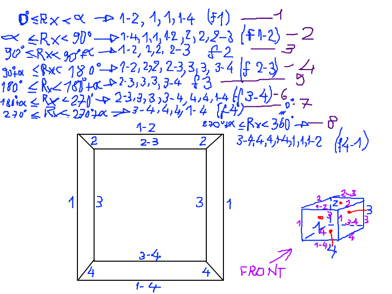
Lines are named using a convention. For instance, lines 1 only belong to face 1. Line 1-2 belongs to both face 1 and face 2. Line 1-4 belongs to both face 1 and 4, and so on. You will see those names in the code that will follow.

The following program performs hidden lines removal by checking the value of the rotation angle. To make things simple, each line is drawn by a subroutine, and the program decides which routines to call on each range of the angle rx.

For instance, as long as rx is less than alfa, the program shows only the first face of the cube. When rx gets more than alfa and it is no bigger than 90 degrees, it shows both face 1 and face 2. But what is alfa? It’s some sort of prospective angle.

If you look at the front view of the cube (those big squares one inside the other, with four short lines joining their vertexes), you will see that between those squares there is a distance. It is due to prospective. The front face is the bigger square, the face opposite to the front face is the small square. If we start rotating the cube, we will start to see face 2 only when the rotation angle gets bigger than the prospective angle alfa.

DOWNLOAD: 3d cube, x-axis rotation, hidden lines (prg file)

DOWNLOAD: 3d cube, x-axis rotation, hidden lines (source code)

 

 

The program just lets you see two faces at a time. It is not that exciting, but at least it shows off this hidden lines removal technique. I have used more values for the trig tables. As a result, motion is slower but smoother, so that you can better see how things work.

In the code, you’ll notice that angles values required some adjustment. This is due to the approximation of integer math using small numbers.

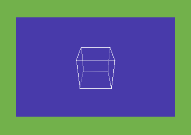
Just to provide you with something a bit more interesting, I decided to draw hidden lines using dot-dot style. This somewhat provides a better rendering of the cube, but the above mentioned optic illusion can still happen.

Dot-dot lines are obtained with a simple modification of the point plotting routine. A flag is switched on and off continuously by using the EOR instruction. Bits are not turned off, plotting is simply skipped. This is not the general way to do it, but it works here.

 

DOWNLOAD: 3D cube, dot-dot hidden lines (prg file)

DOWNLOAD: 3D cube, dot-dot hidden lines (source code)

 

 

I also tested my routines with a pyramid. A slower version with smoother movement (obtained by using more values for trig tables) is also provided. This shape is easier to render and doesn’t seem to suffer from aliasing problems.

 

DOWNLOAD: pyramid (prg file)

DOWNLOAD: pyramid (source code).

 

DOWNLOAD: pyramid smoother (prg file)

DOWNLOAD: pyramid smoother (source code)

 

 

Some notes on performances. Double buffering technique

The programs presented here are by no means fast. They make use of a fast 8 bit multiply routine, but still, they do not use an overall rotation matrix for rotations. Such a matrix allows to perform rotations about all of the three axis quickly. Furthermore, if we write the rotation matrix in a proper form, we can just completely avoid multiplications for rotations. This is shown in the article “A different perspective: part 1” in the Issue 8 of Commodore Hacking. Still, I didn’t use that approach as I wanted to keep my programs simple.

Many things can be optimized in my programs. For instance, zero page could be used for faster access to data. Furthermore, some routines could be improved by using internal CPU registers instead of memory locations, when possible. This code has been written for clarity rather than for speed, but once concepts are clear, code may be changed according to your needs.

Also, a software bitmap screen using programmable characters can be created. That may allow for better performances when plotting points. As only a small part of the bitmap screen is actually used, programmable characters may be enough for that. Again, this is the approach used in the program presented by Commodore Hacking.

Although my routines are slow, no flickering seems to happen. In fact, I have coded a double buffering routine.

Suppose we only use one screen to animate an object. Also, suppose that the animation is quite complex and it can’t be done in a single frame.

If we draw, let’s say, frame1 of the object, then we clear the screen and we draw frame 2, of course we will see some flickering. To get around this problem, we must use two screens, that is, two buffers. Hence the double buffering name.

The programs use the following method. At the beginning, both buffers are cleared. Then, buffer 1 is shown. Buffer 2 is hidden, but it is used for plotting. Thus, buffer 2 is cleared and a frame is drawn on it. Only when the frame has been fully drawn, buffer 1 is hidden and buffer 2 is shown. At this point, buffer 1 will be used for plotting. Again, buffer 1 is cleared, then the frame is drawn on it. Once the drawing process is complete, buffer 2 is hidden and buffer 1 is shown again. This way, images are hidden while they get updated, and they are shown only when they are complete. This way, no flicker can happen.

As switching between the two buffers may cause some very short flickers (due to VIC-II settings changes), buffers must be switched only when the rasterbeam is out of the viewable area. I used a simple busy waiting code to accomplish this. Again, this is not very efficient, but this way code is simple.